| Keypoint | Coordinates (x,y) |
|---|---|
| 1 | (0,0) |
| 2 | (800,0) |
| Key point No | X | Y |
|---|---|---|
| 1 | 0 | 0 |
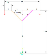
| 2 | 1200 | 0 |
| 3 | 4200 | 0 |
| 4 | 5100 | 0 |
| 5 | 6000 | 0 |
| 6 | 0 | 100 |
| Circle | WP X | WP Y | Radius |
|---|---|---|---|
| 1 | 100 | 50 | 10 |
| 2 | 100 | 100 | 10 |
| Parameters | Path Point Number | X Loc | Y Loc | Z Loc |
|---|---|---|---|---|
| 1 | 50 | 0 | 0 | |
| 2 | 50 | 150 | 0 |
| Keypoint No. | X | Y |
|---|---|---|
| 1 | 0 | 0 |
| 2 | -20 | 0 |
| 3 | -20 | 100 |
| 4 | 0 | 100 |
| 5 | 0 | 95 |
| 6 | -15 | 95 |
| 7 | -15 | 5 |
| 8 | 0 | 5 |
| Keypoint | Coordinates | ||
|---|---|---|---|
| x | y | z | |
| 1 | 0 | 0 | -Z1 |
| 2 | 0 | 0 | Z1 |
| 3 | X1 | 0 | 0 |
| 4 | X1 | Y1 | 0 |
| 5 | X1 | Y3 | 0 |
| 6 | X2 | Y2 | 0 |
| 7 | X2 | Y3 | 0 |
| Node Number | X | Y | Z |
|---|---|---|---|
| 1 | 0 | 0 | 0 |
| 2 | 3 | 0 | 0 |
| 3 | 3 | 3 | 0 |
| 4 | 0 | 3 | 0 |
| 5 | 0 | 0 | 3 |
| 6 | 3 | 0 | 3 |
| 7 | 3 | 3 | 3 |
| 8 | 0 | 3 | 3 |
| 9 | 0 | 0 | 6 |
| 10 | 3 | 0 | 6 |
| 11 | 3 | 3 | 6 |
| 12 | 0 | 3 | 6 |
| 13 | 1.5 | 1.5 | 7.5 |
| Type | Description | Visual Representation |
|---|---|---|
| SECT | Section display. Only the selected section is shown without any remaining faces or edges shown | |
| CAP | Capped hidden display. This is as though a portion of the model was cut off and the remaining model can be seen | |
| ZQSL | QSLICE Z-buffered display. This is the same as SECT but the outline of the entire model is shown. |